
We all have been taught in our high school that for a material like metals (steel or iron) they follow a proportional path when it comes to stress and strain or force and displacement. After a certain point, it starts to behave as not proportional (nonlinear). This point is called Yield Point.
Basically, Yield Point is the point where the material properties of hooke’s law doesn’t govern. Stress is not proportional to strain and when the stress is released permanent deformation is seen. So, proportionality limit was analogous to elastic limit.
Elastic limit is the point where upon if the stress in the object is released it is released back to its initial point. For e.g. take an iron rod of 15cm and pull that rod from both sides equally with 1000 N force, and say it becomes 15.3 cm, (the exact value will be far in range of 15.0098 or whatever range, 15.3 is just for reference). And let’s take this force out 1000N, and we can see the rod contracting to be in the same position. If it reaches 15cm. Then the 1000N force is in elastic limit. If not, then it will be plastic limit and the change in the length is called permanent deformation.
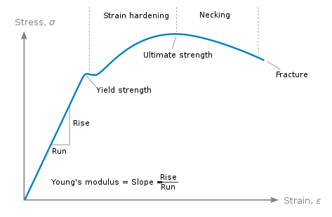
Most common engineering materials exhibit a linear stress-strain relationship up to a stress level known as the proportional limit. Beyond this limit, the stress-strain relationship will become nonlinear, but will not necessarily become inelastic. Plastic behavior, characterized by nonrecoverable strain or plastic strain, begins when stresses exceed the material’s yield point. Because there is usually little difference between the yield point and the proportional limit, the Mechanical APDL application assumes that these two points are coincident in plasticity analyses.
So even for nonlinear region below yield point it is still in elastic limit. If we need to find out the absolute plastic strain reading, we need to locate the elastic limit point, (which is not always the proportional limit). There are two models that we can use in analysis.
- Bilinear Stress Strain Curve
- Multilinear Stress Strain Curve
Bilinear Stress Strain Curve
Two linear line is assumed with two different moduli of elasticity in this model. Many of the software package use this model to analyze non-linearity.
The “von Mises with – Hardening” material model will use a bilinear curve to calculate the stress values. The elastic region of the stress versus strain has a slope equal to the modulus of elasticity, and the plastic region of the stress versus strain has a slope equal to the strain hardening modulus.

Multi Linear Stress Strain Curve
The material behavior is described by a piece-wise linear stress-strain curve, starting at the origin, with positive stress and strain values. The curve is continuous from the origin through numerous stress-strain points. Successive slopes can be greater than the preceding slope; however, no slope can be greater than the elastic modulus of the material. The slope of the first curve segment usually corresponds to the elastic modulus of the material, although the elastic modulus can be input as greater than the first slope to ensure that all slopes are less than or equal to the elastic modulus.
